In Part 1 we covered stacking similar and different plot types in ggplot2 and gridExtra. Unfortunately we ran into limitations that hindered us from creating a complex plot such as a pie charts overlaid on a map (which I won’t exactly cover yet, sorry). To accomplish this we need to dive into the inter-working of GrObs.
GrObs: The Good
GrObs are short for Graphical Objects and form the basis of the Grid graphical package. Don’t worry on installing it, your already have it since it is distributed with R. More so you most likely already use it since it many other packages such as ggplot2 build off it. With out getting into the specifics, everything drawn [in ggplot2] are GrObs and hence there is an easy function to create one: ggplotGrob(). Now if only there was a simple way to add a GrOb to an existing plot.
Well thankfully ggplot2 gave us this functionality with annotation_custom(grob, xmin, xmax, ymin, ymax). The function takes a GrOb and places it in a plot (bounded by X/Y min/max). A nice additional feature of this is that the coordinates are defined by the plot coordinates and not the display’s. Let’s see this in action.
We will start with these three plots depicting the distribution of transmission type per number of cylinders.
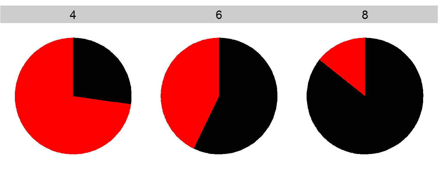
Note that this was plotted with facets, however we want to store the plots as individual objects. We do this via
cyl.pie <- function(c){
    ggplot(data = count(subset(mtcars, cyl == c), "am"),
	   aes(x = "none",
	       y = freq,
	       fill = factor(am))) +
	geom_bar(width = 1,
		 stat = "identity") +
	coord_polar("y") +
	scale_fill_manual(values = c("0" = "black", "1" = "red") +
	theme_nothing)
}

pies <- alply(c(4,6,8), 1, cyl.pie)
names(pies) <- c(4,6,8)
cyl.pie() should be pretty self explanatory since it simply creates a pie chart for the particular cylinder subset of mtcars(). From there we simply create a list of each pie chart per cylinder (and rename it for easy access. Two things need attention:
- The X aesthetic needs defining even though it is not used (x = “none”) and may be due to my own ignorance.
- theme_nothing which is borrowed from the ggmap package.
theme_nothing <-
    theme(axis.text =          element_blank(),
          axis.title =         element_blank(),
          panel.background =   element_blank(),
          panel.grid.major =   element_blank(),
          panel.grid.minor =   element_blank(),
          axis.ticks.length =  unit(0, "cm"),
          axis.ticks.margin =  unit(0.01, "cm"),
          panel.margin =       unit(0, "lines"),
          plot.margin =        unit(c(0, 0, -.5, -.5), "lines"),
          plot.background =    element_blank(),
          legend.position =    "none",
          complete = TRUE)
Basically it strips everything off of the plot. Note that plot.background = element_blank()has been added which assures that the plot has absolutely nothing behind the pie chart (typically this is white and not noticed).
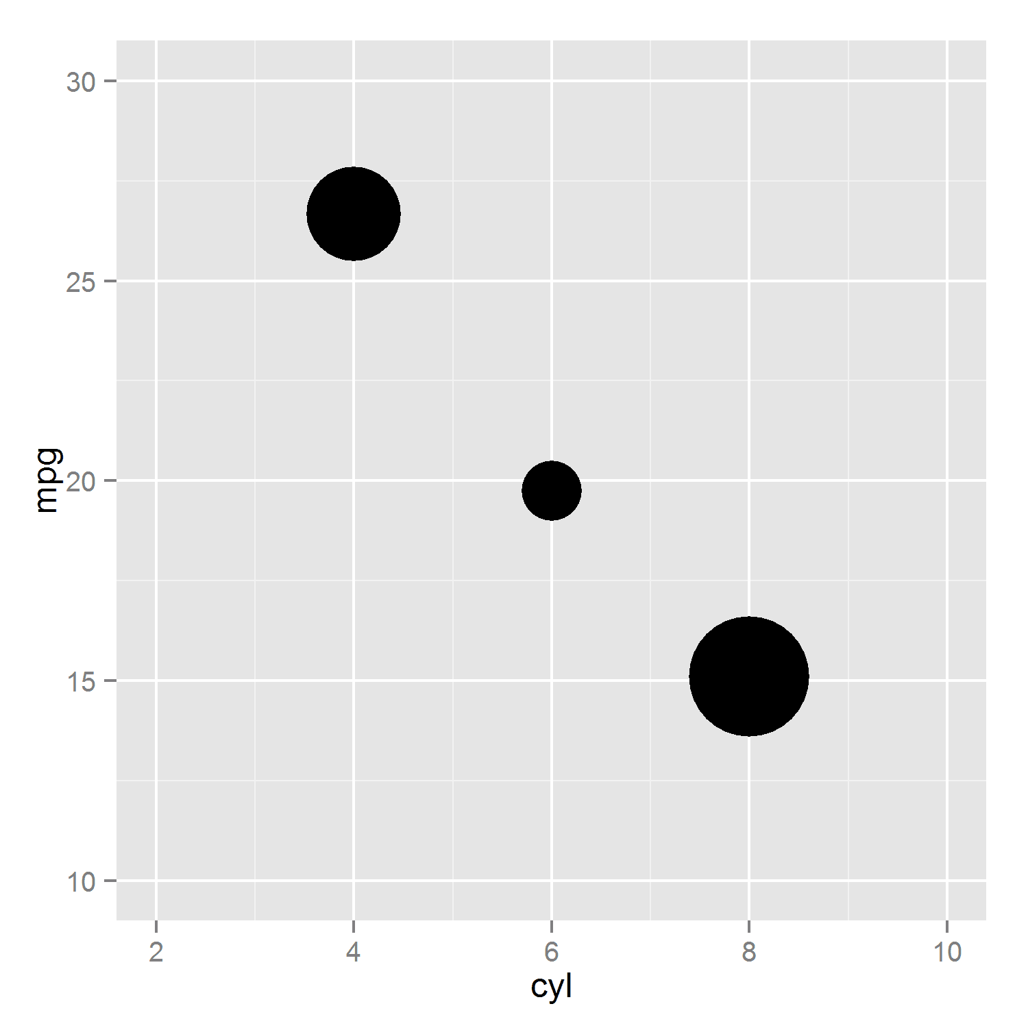
Next we need another plot to put these pies into. I will choose the average MPG vs the number of cylinders with the addition of sizing the groups based on the number of cars.
and code generating this
super.plot <-
    qplot(data =
          ddply(mtcars, .(cyl),
                summarize,
                mpg = mean(mpg),
                n = length(cyl)),
          x = cyl,
          y = mpg,
          size = n) +
    scale_size_continuous(range = c(10, 20)) +
    theme(legend.position = "none") +
    xlim(2, 10) +
    ylim(10, 30)
So as I mentioned, to add the subplots we simply need to convert them to GrObs and append them like so:
super.plot +
    annotation_custom(ggplotGrob(pies[["4"]]),
                      3, 5, 24.5, 28.5) +
    annotation_custom(ggplotGrob(pies[["6"]]),
                      5, 7, 18.5, 21) +
    annotation_custom(ggplotGrob(pies[["8"]]),
                      7, 9, 12, 18)
And viola
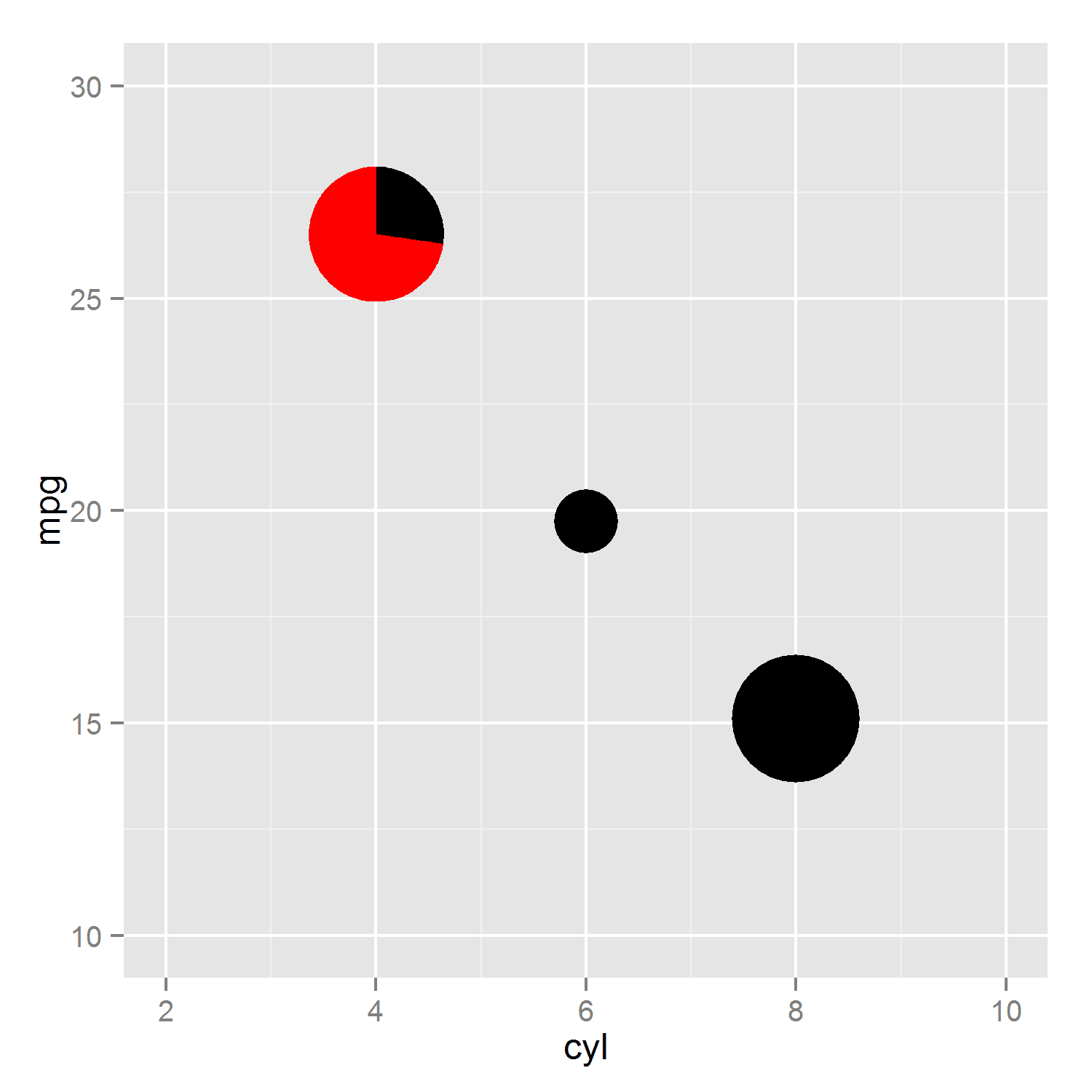
Wait! What?!?!
GrObs: The Bad
So what happened here. Well first we took our original plot and annotated a GrOb of the 4-cylinder pie chart between cylinders 3-5 and MPG 24.5-28.5. Notice that the pie is correctly scaled even though it should be wider than it is taller. Next we should be plotting the 6-cylinder pie at 6, 20 and the 8-cylinder pie at 8, 15, but where are they?
Well it takes a little digging but the issue lies in how ggplot2 keeps tracks of GrObs. When we convert a plot to a GrOb, ggplotGrob()gives it a name. It always names the GrOb ‘layout‘ no matter what. Now when ggplot2 draws objects, it likes very unique names. There is probably good reason for this, so don’t go pestering Wickham, however since ggplot2 already drew ‘layout‘ once (this being the 4-cylinder pie) it does not draw the subsequent ‘layout‘ GrObs (the 6 & 8-cylinder).
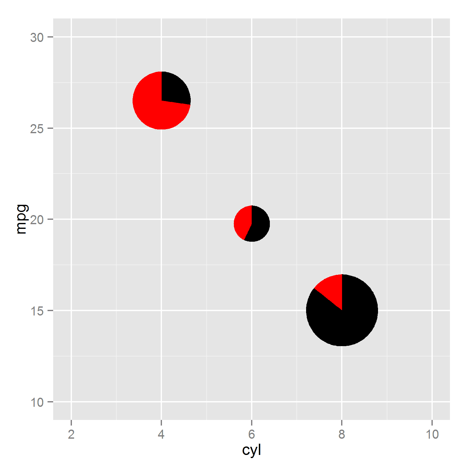
Let us fix this by changing the names:
pies.grobs <- llply(pies, function(g) {
    g <- ggplotGrob(g)
    g$name <- paste(g$name, sample.int(10^9, 1))
    g
})

super.plot +
    annotation_custom(pies.grobs[["4"]],
                      3, 5, 24.5, 28.5) +
    annotation_custom(pies.grobs[["6"]],
                      5, 7, 18.5, 21) +
    annotation_custom(pies.grobs[["8"]],
                      7, 9, 12, 18)
GrObs: The Beautiful
So there you have the basics. Honestly all that is needed is some clean up. For instance:
- A function to place them in the right place and with the right size
- Some way to add a legend
sub.plot.locations <-
    ddply(mtcars, .(cyl),
          summarize,
          mpg = mean(mpg),
          n = length(cyl))

super.plot <-
    qplot(data = sub.plot.locations,
          x = cyl,
          y = mpg,
          size = I(2),
          color = I("dark grey"),
          geom = "line") +
    geom_text(aes(label = paste("n =", n),
                  y = mpg - n/7 - 0.3)) +
    theme(legend.position = "none") +
    xlim(3, 9) +
    ylim(10, 30)

Add.Sub.Plots(super.plot,
              pies,
              as.character(sub.plot.locations$cyl),
              sub.plot.locations$cyl,
              sub.plot.locations$mpg,
              sub.plot.locations$n / 75) +
    annotation_subplot(Plot.Legend.Fill(c("Manual", "Automatic"),
                                        c("red", "black"),
                                        bg.color = "white",
                                        text.color = "black"),
                       7.5, 25, 1)
yielding
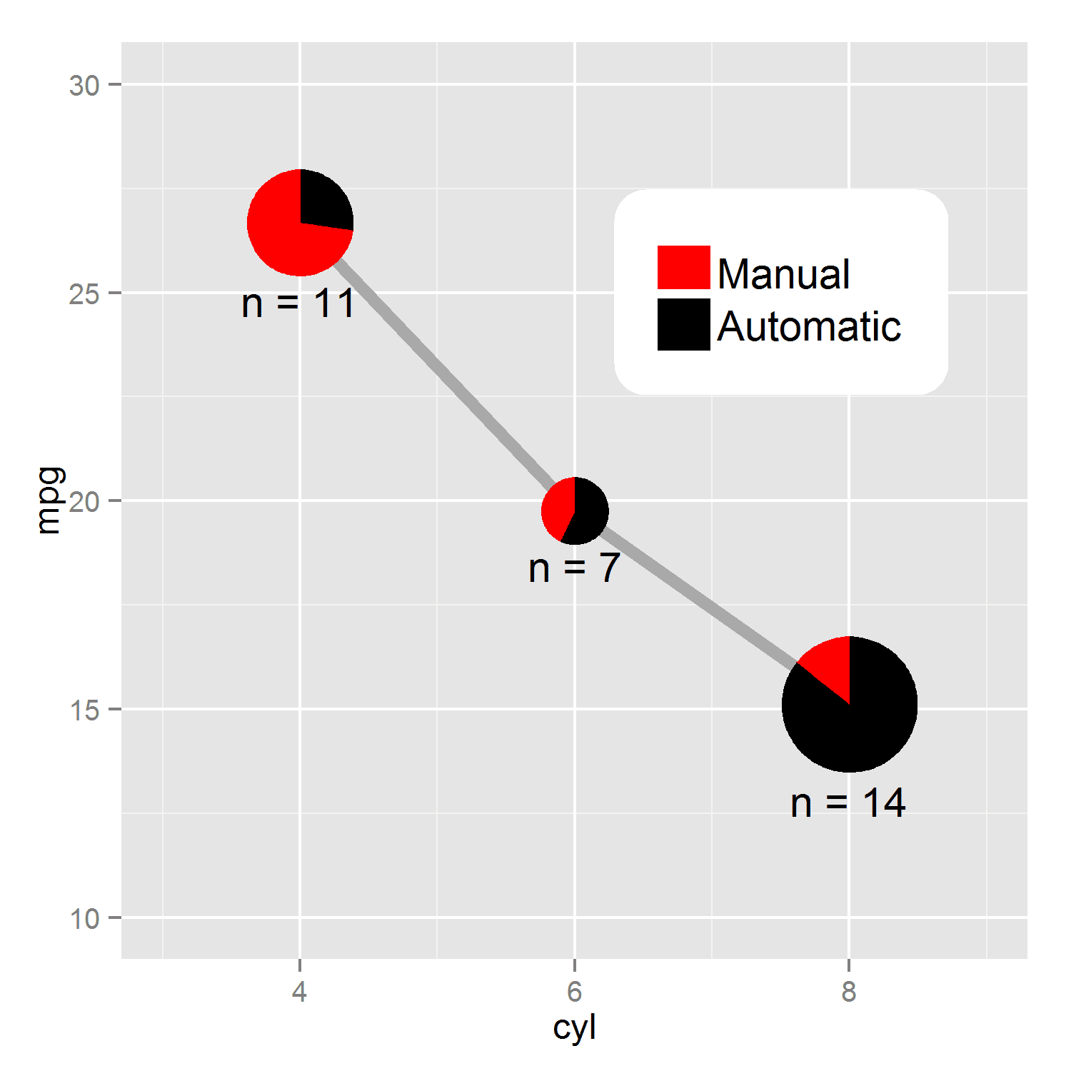
Which oddly now begs the question: are V8s less efficient because they are big or because they typically have an automatic transmission?